After completing four projects for the Flatiron Data Science course, I discovered that one aspect of data exploration (Exploratory Data Analysis or the E of OSEMN) that I enjoy is feature engineering.
Feature engineering involves thinking critically about a dataset with the purpose of re-imagining variables to get a desired quality or form. For example, one might consider how text variables might become categorical or numerical variables. It could be based on counting the number of characters or separating a list that was stored in one variable into multiple dummy columns. This blog post will review two features I engineered, each for a different project.
Getting the winter season in Module 3
(Project slide deck available at this link.)
The project prompt was to formulate and test four hypotheses on the Northwind SQL database. It contains several tables with sales information for the fictional Northwind company. Once I knew I wanted to compare shipping details for different orders, I could use the date of a shipment to determine what the weather was like for that order. It would be simplest to implement by using season as a proxy for the weather and then my alternate hypothesis was whether freight costs were different for wintry weather (defined as orders that occurred during meteorological winter). I used the date to determine which meteorological season the shipment occurred in. However, since orders were shipped to the Americas and Europe, I also needed to account for the fact that the Southern and Northern Hemisphere have their seasons opposite from each other.
I first added the Hemisphere column for whether the ShipRegion was in the Southern or Northern Hemisphere. One value that I needed to be sure of was “Central America” but a majority of that region is in the Northern Hemisphere. This left “South America” as the only ShipRegion in the Southern Hemisphere.
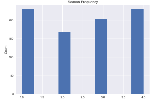
Next, I wrote code to classify the dates by meteorological season based on which three-month period the record fell into and which value it had for Hemisphere. This used a series of if statements comparing months for seasons (March-May, June-August, September-November, December-February) in a function which_season, returning numbers 1 to 4, with 1 for Spring. Below is the Southern Hemisphere half of the code from which_season, followed by the call creating the Season column in the ordersdf dataframe with a list comprehension.
else:#if Southern Hemisphere
        if 3<=month<6: #between March 1 and June 1, excluding June 1
            return 3 #3 for Autumn
        elif 6<=month<9:
            return 4 #4 for Winter
        elif 9<=month<12: #between September 1 and December 1
            return 1 #1 for Spring
        else:
            return 2

ordersdf["Season"] = [which_season(date.month, hemi) for date, hemi in zip(ordersdf.ShippedDate, ordersdf.Hemisphere)]
Finally, I sampled the Season feature to get two lists of freight costs, based on whether the record had the number 4 or not:
winter=[x for x, y in zip(shipdf["Freight"], shipdf["Season"]) if y==4]
notwinter=[x for x, y in zip(shipdf["Freight"], shipdf["Season"]) if y!=4]
Combining rare dummy features for Module 5
(Module 5 project repository available here.)
Another piece of code I enjoyed working on was for a dataset of details about strategy game apps (from a Kaggle user), where three features were stored as strings listing values: Subgenre, Language and In-app Purchases. Although I did not make use of the code in my final model, the resulting engineered feature from this dataset was interesting to consider.
After separating out the lists within those particular features to become dummy columns, I noticed that many dummy columns had few entries. For example, Weather was a very unusual subgenre for a strategy game app.
I wrote a function to take in a dataframe of purely dummy columns for the same feature and return it with a new column with “etc” in its name that combined all of the dummy columns below a given threshold of non-null values. This new column was also a binary feature with 1 when a record fell into any one (or more) of the specified less-frequently appearing dummy columns.
First, it found whether a column had more non-null values and added it to a list of column names, using isna() and given a number threshold for how many non-null entries a column would need to have to not be combined into the new “etc” column.
hold=len(dataframe.index)-threshold #acceptable number of null values
    for colname in dataframe.columns:
        totalnull = dataframe[colname].isna().sum() #finding how many NaN entries in a column
        if totalnull > hold: #if the column has more than the acceptable number of null values
            colcombine.append(colname)
Then, the function loops through each record, looping through each column for it in colcombine. If the current column from colcombine has a 1 at that index, the “etc” column at that index is set to 1.
try:
     if(dataframe.loc[idx,col]==1):
           dataframe.loc[idx,prefix+"_etc"]=1 #sets that index position in "etc" to be 1
except: #if the location is null, go to next column in colcombine
      continue
When I ran it on Subgenre columns, I found that even collecting the dummy columns that had fewer than 100 entries (if fewer than 100 records had that subgenre listed) resulted in a column with 600+ records. This was less than a tenth of the dataset but more than the new least-frequently appearing subgenre, with 188 records. Ultimately, I did not use this function and left the Subgenre categorical variable as individual dummy columns so all of them could be taken into account when determining feature importances.