One important concept of data science that comes up in this course is overfitting and underfitting. Overfitting is when a function fits the training data supremely well, to the exclusion of any other data. LASSO (Least Absolute Shrinkage and Selection Operator) and Ridge regressions or (L1 and L2 Norm Regularizations, respectively) are two related approaches to overfitting and are used similarly to a linear regression model. They use a hyperparameter to penalize the coefficients so some are zero or closer to it in order to filter out noise in the data, thus helping reduce overfitting.
These regressions (also called regularizations) are implemented with the Python package sci-kit learn and can be imported with from sklearn.linear_model import Ridge, Lasso and then initialized with Ridge() and Lasso().
LASSO and Ridge regressions provide useful results for standardized data. Since they rely on penalizing coefficients, differences between the scales of feature variables will become exaggerated if the data has not been standardized. In other words, variables that consist of larger numbers would be treated as more important. One way to scale the data is with scikit-learn’s standardization method accessed with from sklearn.preprocessing import StandardScaler.
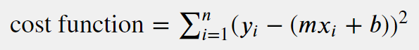
The cost function (also known as a loss function) for solving for a linear regression is:
A LASSO regression cost function looks like:

LASSO regression is based on ordinary least squares regression. Its regularization hyperparameter λ (a.k.a. penalty term) needs to be set before estimating the parameters through the training algorithm. The absolute value of each coefficient in the cost function is multiplied by the penalty term. LASSO allows for coefficients to shrink to exactly zero, which reduces the amount of calculations because the regression eliminates the feature associated with those coefficients.
Using sci-kit learn:
reg = Lasso(alpha = sparsity)reg.fit(X,y)predictions = reg.predict(datapoints)
The parameter alpha is a float between 0 and 1. If it is set to zero, Lasso is equivalent to ordinary least squares and the documentation encourages using the LinearRegression object instead. Specifically, the warning text says the “algorithm does not converge well.” The larger alpha is, the more features will not be selected, as more coefficients shrink to zero.
Scikit-learn has several other kinds of LASSO models, available to peruse here.
A Ridge regression cost function may be represented by:

For Ridge regression, each coefficient in the cost function is squared and then multiplied by a penalty term λ. For small λ’s, the ridge regression will be close to a linear regression model. For a larger λ, the larger coefficients penalize the cost function and have a greater effect on the optimization, because more of the coefficients are smaller and shrink their respective features.
In scikit-learn, alpha is the strength of the regularization and must be a positive float (or a numpy.ndarray of positive floats, one for each target). A higher value for alpha means the stronger the regularization and the smaller more of the coefficients, shrinking more of the features. Similarly to Lasso, with an alpha at zero, the solution is more like ordinary least squares regression.
In Python:
reg = Ridge(alpha=strength)reg.fit(X, y)predictions=reg.predict(datapoints)
Two other related objects: classifier RidgeClassifier and ridge regression with cross-validation RidgeCV can be found at this link.
Both the Lasso and Ridge objects can be initialized by specifying more parameters besides alpha, including: a limit to the number of iterations max_iter, a tolerance for optimization tol (for Ridge this is solution precision; Lasso uses a coordinate descent algorithm), and the boolean normalize which normalizes X before performing the regression if set to True.
In addition, the Lasso object has an option warm_start to reuse the solution of the most recent call as its initialization. The Ridge object has a solver argument with several options, among them: auto, the scipy.sparse.linalg.lsqr regularized least-squares lsqr, and a Stochastic Average Gradient descent saga. As mentioned above, Lasso uses a coordinate descent algorithm.
The Lasso and Ridge objects have the same attributes: the coefficients coef_ (a numpy ndarray corresponding to the m’s in the cost function), the intercept_ (corresponding to the b’s in the cost function) and n_iter_ number of iterations that were needed to meet the tolerance. The one exception is that Lasso also has sparse_coef_. Since coefficients in LASSO regression can be zero, it returns an array of the nonzero coefficients and coordinate pairs of their feature locations. For instance, if X was three features, y was one target and the second coefficient was the only one not shrunk to zero, sparse_coef_ would return (0,1) and the value of that second coefficient.
The ability of the hyperparameters to affect the coefficients in both LASSO and Ridge is what can help with overfitting, since the idea is to select coefficients so as to minimize noisy features and maximize important ones. A cost function’s coefficients and hyperparameters may be built on existing data with the expectation of applying it to future data so it’s also important to consider whether the regularizations are too strong. Evaluating with test data to find an appropriate balance in linear regressions and with alpha (or λ) hyperparameters adjusting the impact of the coefficients can address this challenge.
Thanks to The Flatiron School, Inc. and the scikit-learn documentation for informing my understanding.