Module 4 Final Project

The fourth module of the course introduced time series.  The final project for it asked me to make use of time series analysis techniques to identify which zip codes from a given dataset of house prices would be the best five to invest in.

I determined that a top zip code would be one where the housing market collapse in 2007-2008 did not affect the prices very much.  It would also be located near zip codes that had seen a price increase in the past few years because that may indicate the county itself is doing better financially and would be more desirable area in which to live.  Thus, these factors would indicate that a house price would be more likely to increase in the next few years.

The data was from sales prices recorded on Zillow in the United States and dated by month from April 1996 to April 2018.

One of the first realizations I had was that my hypotheses or criteria for investment were beyond my studies of time series-based analysis in Module 4. After looking over relevant labs and reading through the provided starter notebook, I decided to find the model and corresponding parameters that best described an average of all of the prices data, by month. I would then use that information to determine which records most closely matched the model and make predictions for those records, with the best zip codes having the best results.

For a while, I tried to make my data stationary before running a model. After a few attempts, I decided to use the SARIMAX model from the statsmodels package, as that does not rely on starting with detrended data.

The next adaptation I needed to make to my plan was to account for how long it would take to model and generate predictions for however many records I was considering. After timing runnning the code to evaluate the model in different ways for a few records, I calculated that, at worst, it could take over 100 days to evaluate the model for every record. I endeavored to reduce it to 8-10 hours.

As I had chosen the SARIMAX model because it was the best fit for the data, the running time could only be reduced by lessening the number of predictions. My resulting analysis consisted of a subset of the data, specifically the middle ninth (between the 44th and 55th percentiles), comparing the first five values forecasted with the model using the training set to the corresponding known first five values of the test set. I used the lowest mean-squared error as a guideline to choose my next subset of records.

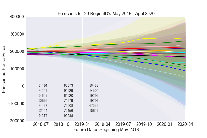
Practically, modeling and predicting for the twenty records with the lowest mean-squared error would not take an incredibly long time. With those 20 selected records, I ran the model again and made forecasts for 24 steps ahead (corresponding to two years) until April 2020 for each record.

I then chose to compare the lower bounded values of the 95% confidence interval in April 2020 to the latest actual value from April 2018. The five records with the highest percent changes by this comparison became the five recommendations. Through the proxies for a safe bet, those were the least likely to lose the largest amounts of money.

I would also add that I am reluctant to single out the cities and counties by name on the World Wide Web, especially when my analysis is not as accurate as I know it could be.

Some observations I would take into account when doing a similar project in future:

1. I would seriously consider that house prices are very unlikely to be sold for negative amounts in the real world and try to account for this in the model.
2. House prices could vary by many factors, some of which are measurable by Zillow so it may be worthwhile to draw from government databases on zoning, for example, or monthly overviews of the weather.
3. It would be great to compare the expected Return On Investment to any insurance policies, mortgage payments, agents’ fees, rental income and other expenses that may be necessary when reselling property.
4. A more balanced picture of the predictions would involve looking at the upper bound of the confidence interval and over different stretches of time.
5. Timing every step to determine how long each part takes is helpful in getting a feel for whether an idea can reasonably scale to the entire dataset.
6. Of course, I would still like to test my original hypothesis: that the best places to invest would be those that went through the housing market collapse relatively unscathed and/or were nearby areas that had recently experienced an increase in prices.